


Everything You Need to Know about Landsat Satellite Imagery

Nikhil Hubballi

12 minutes
Spatial Analytics
Explore a New Open Dataset Every Week - Week 1 - Landsat
Satellite imaging is one of the breakthroughs of the 20th century. Started as the race to display supremacy over space domain between the US and the USSR during the cold war, soon turned into an essential science to help observe the earth regularly to understand terrain changes, forecast weather, increase agriculture productivity, land use mapping for city planning and many more applications.
Today, there are hundreds of private sector companies along with government-funded space agencies that are building new satellites to capture the earth's surface and atmosphere in near-real-time. Although many of the data from the govt. agencies are available on public domain for free to use in scientific areas, many of the more granular datasets are licensed.
There's one mission with multiple satellites in the public domain that's providing free and reliable satellite imageries at high-resolution for almost 5 decades, called Landsat. In this blog, we look into Landsat Satellite Imagery, its use cases over the years along with how you can get the data yourself and get started on processing & visualizing the data.
This blog is the first in the series of exploring a new open dataset every week. Stay tuned for the upcoming blog on Sentinel 2 next week.
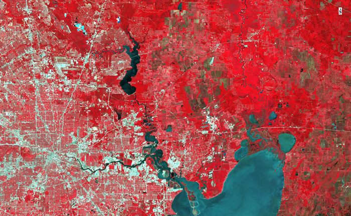
featured image: Infrared Image of the city of Houston, USA, captured using Landsat 8; tnris.org
What's Landsat?
A brief history
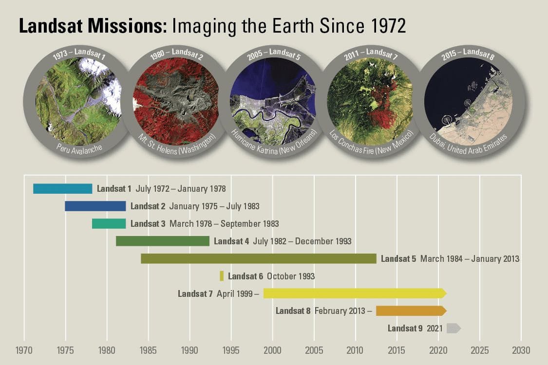
Started as the Earth Resources Technology Satellite on July 23, 1972, Landsat is the longest-running satellite imagery mission. Landsat mission was initiated at the NASA's Goddard Space Flight Center but after the launch of the 3rd Landsat satellite in 1979, the operations of the mission were transferred from NASA to NOAA with a plan to conceive a long-term operational system.
But soon the mission faced funding issues for continued satellite launches and the launch failure of Landsat 6 in the mid-1990s affected the mission's survival. Understanding the value of the Landsat missions there was a Land Remote Sensing Policy Act (Public Law 102-555) in the US congress that helped the future mission of Landsat 7 in 1999, the 2nd longest-running Landsat Satellite after Landsat 5, with state-of-the-art sensors for satellite imaging.
Landsat satellite imagery has helped in numerous scientific and commercial applications all over the world since its inception and has become a go-to dataset with its regularly updated and short-temporal, high-resolution imagery for the entire globe.
Technical details
Landsat 8 is the latest satellite in the mission that was launched in 2013. It has two imaging sensor payloads, Operational Land Imager (OLI) and Thermal Infrared Sensor (TIRS). OLI has 9 spectral bands that span from visible blue wavelength to short-wave infrared along with a panchromatic and cirrus bands and TIRS has 2 thermal bands.
With a repeat cycle of 16 days, Landsat 8 captures around 740 scenes a day across the globe. Each scene is approximately 180x180 km in size in the path/row system of Worldwide Reference System-2 (WRS-2). Master shapefile for WRS-2 path/row scene tiles for the whole globe is available here.
Check out more details on the technical details of previous satellite missions here.
How to get the data?
The Landsat data is currently managed by NASA and the United States Geological Survey (USGS). The data is accessible through 3 different data portals handled by USGS, EarthExplorer, Global Visualization Viewer (GloVis) and LandsatLookViewer. And NASA provides the Landsat data through its EarthData portal. For most use cases using Landsat, a Level-1 product (terrain corrected) can be used. This product typically includes data from both OLI and TIRS sensors. Individual sensor scenes are available as well in the archive.
The first two values of the Landsat 8 product ID designate the data provided in each scene, with Tier 1 being the high-precision terrain corrected scenes:
In Level 2 scenes derived using Landsat, Top-of-Atmosphere Reflectance, Surface Reflectance, Surface-reflectance based spectral indices like NDVI, and NDMI are major products.
Using Online Portals
There are two popular methods to download Landsat 8 – L1 scenes from online portals. One using the EarthExplorer and another from EarthData. We will look at both the methods here.
1. USGS - Earth Explorer
You need to create an account with USGS on EROS Registration System (ERS) to be able to download the Landsat satellite imagery data from EarthExplorer. Create and activate your account by following the procedure on the portal. The portal allows searching the data based on date periods, criteria for bounding box, scene identifiers (path/row numbers), max cloud cover etc.
The downloading process involves 4 simple steps.
- Set Area of Interest on the map for search criteria
- Choose the dataset to be downloaded
- Apply additional criteria to the data
- Check the results and download
The complete steps involved in getting the data from EarthExplorer can be found in this blog from GIS Geography. Even though earth explorer is easy to use, setting up bulk downloads is time-consuming. NASA's EarthData provides an easy solution for this.
2. NASA - EarthData
First, you'll have to create an account with NASA's EarthData. Once registered and activated, log into your account. Downloading the data from EarthData involves similar steps as for the EarthExplorer.
STEP 1: Search Dataset and Set Search Criteria
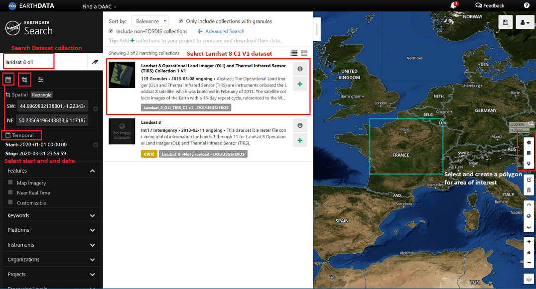
Set your area of interest by choosing the create polygon button on the right of the map and drawing a polygon on the map. Choose the start and end dates for your search. Then choose the dataset by searching for 'Landsat 8 oli' and choosing the Landsat 8 OLI/TIRS Collection 1 Version 1 product from the dataset collections.
Alternatively, for the area of interest, you can also supply a point or a kml/shapefile by clicking on the crop icon on the left below the search box.
STEP 2: Apply Additional Criteria
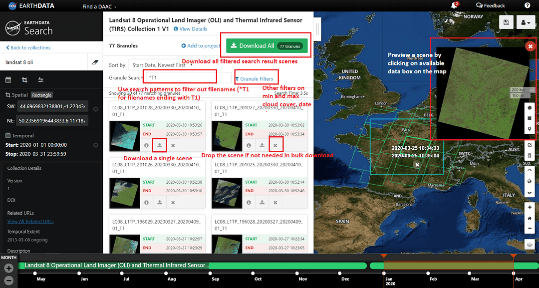
Once the dataset is selected, you are shown the search results with available scenes for the area of interest selected in the date range. Now, you can add more criteria to filter results. Since we need a high-precision terrain corrected data product of Landsat, we filter for filenames that end with T1. We can also add other granule filters such as minimum and maximum cloud cover allowed for scenes. If any particular scene from the search result is not needed it can be dropped individually.
Once we are satisfied with the search results, we can proceed to download all available scenes for the search criteria with applied filters.
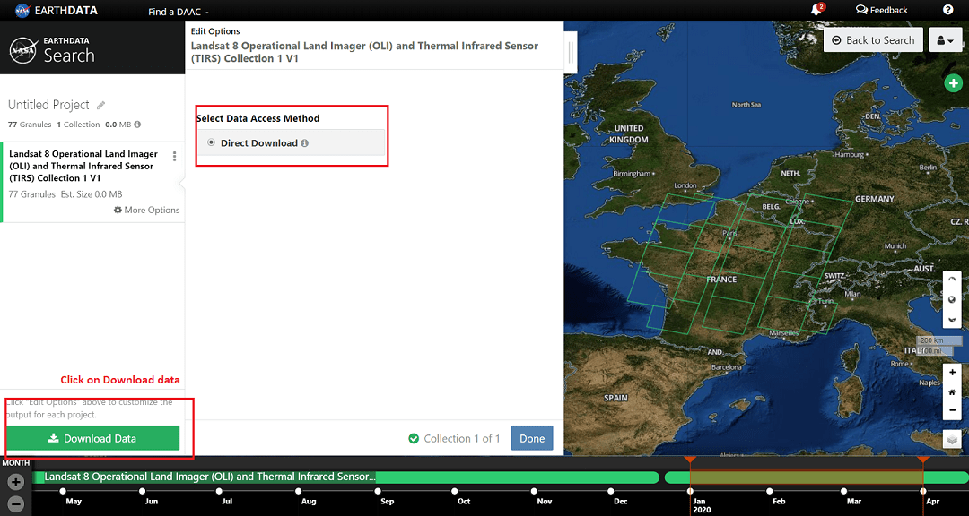
STEP 3: Confirm the order status and Download
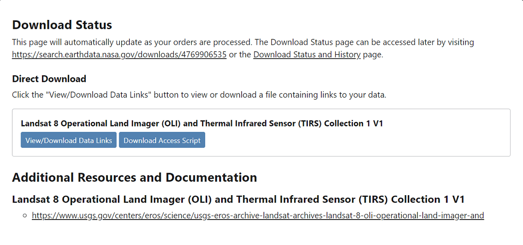
Once the order is submitted and processed, you will be provided with an option to download a text file that contains all the Landsat scene links along with another option to download a bash script to run on the terminal and download the data.
To download the data using the links text file, run the following code from your terminal, where myusername is your Earthdata username, mypassword is your Earthdata password, and url_list.txt is a text file with one granule download link per line.
If you choose to download the data using the script file instead, download the script file and make it executable before running it. The script will ask for your Earthdata Login credentials which are case-sensitive.
Using CLI
Development Seed, a company that works on building open-source software tools for GIS and big data, introduced a command-line utility tool in 2014 for searching, downloading and processing Landsat imagery.
Instead of the USGS EarthExplorer, it uses the Landsat data stored on the google cloud storage platform to download the data faster. Google has partnered with NASA and USGS to host the Landsat imagery and provide it to the public for free through its Google Earth Engine project.
Installing
Run the following commands from your terminal -
On Mac-OSX:
On Ubuntu:
Once installed, check if the utility works by running landsat -h, it should display the manual and parameters to use the tool.
Searching
The tool uses landsat-api (now sat-api) to search the Landsat 8 scenes by using search criteria such as date range, max cloud cover percentage and choosing the geographic region either by path/row id or a latitude, longitude pair.
To search by path and row, add the search parameters as below -
Search by latitude and longitude using the command below -
The search results would contain all the Landsat scenes with unique IDs that match the criteria. These IDs can be used to download using the next step.
Downloading
Searching for the Landsat scene provides the search results with scene IDs which can be used to download using the landsat-util. Choosing a unique ID for the download will get all the bands into a zipped file. If only certain bands are required, they can be specified before downloading.
Download images by their custom scene ID, which you get from Landsat search:
To download only bands 4, 3 and 2 for a particular scene ID run:
Download multiple scene IDs:
For more details on the landsat-util module and its usage, check out the docs.
Using Python
Similar to landsat-util, there's another tool available known as landsatxplore. This also allows a command-line utility tool to search and download the Landsat data collections. You can also use this through the python API so that you can integrate it into your already built python workflows. Unlike landsat-util, this tool uses Earth Explorer JSON API to search for scenes.
Install the tool using pip.
Search for scenes using the Earth Explorer API.
Download the retrieved scenes
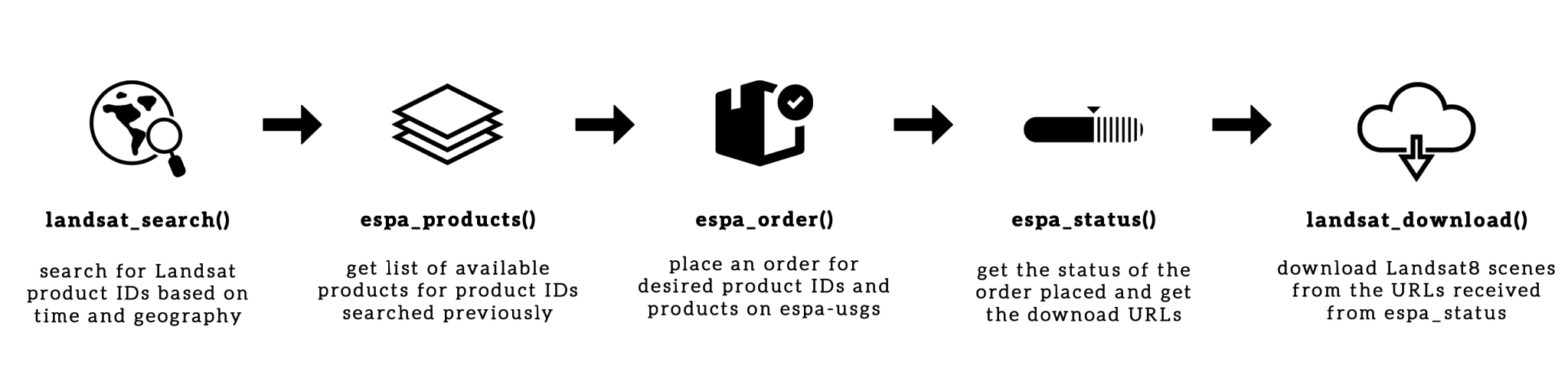
Using R
Using the sat-api from Development Seed and the espa-api from USGS-EROS, there's an open-source package on R called rLandsat. A previous colleague of mine from Atlan, Himanshu Sikaria built this very intuitive tool that simplifies the process of searching for Landsat 8 products, placing the order and downloading the data. Meta-information for the dataset is available from AWS S3 Landsat 8 metadata.
Install the rLandsat package from R using the following command.
Example code to search for the Landsat Product, order and download.
Visualizing the Landsat scenes
Requirements: GDAL - a GIS toolkit to manipulate raster and vector data, Matplotlib, Numpy, Rasterio, Earthpy
We have already looked at how to get the Landsat satellite imagery data for any area of interest. Here, we have fetched the data for the Mumbai region for the most recent available scene with product ID LC08_L1TP_148047_20200311_20200325_01_T1. Here, LC08_L1TP at the beginning of the product ID represents Landsat 8 Combined (OLI & TIRS) Level-1 Terrain precision data product, while the next 6 characters '148047' describe the path (148) and row (047) for the scene.
The product file for each scene is a '.tar.gz' file that contains all the spectral and thermal bands along with a Quality Assessment (QA) as GeoTIFF images and a meta file for the data product. Each of the compressed scene products is significantly large as high as 1GB. This Level-1 Terrain corrected data is a standard beginner product for most of the use cases based on Landsat 8.
Import necessary python modules for visualizing the Landsat satellite imagery.
Fetch a list of all the spectral bands and create a stacked raster consisting of 7 spectral bands from ultra blue to short-wave infrared.
Output:
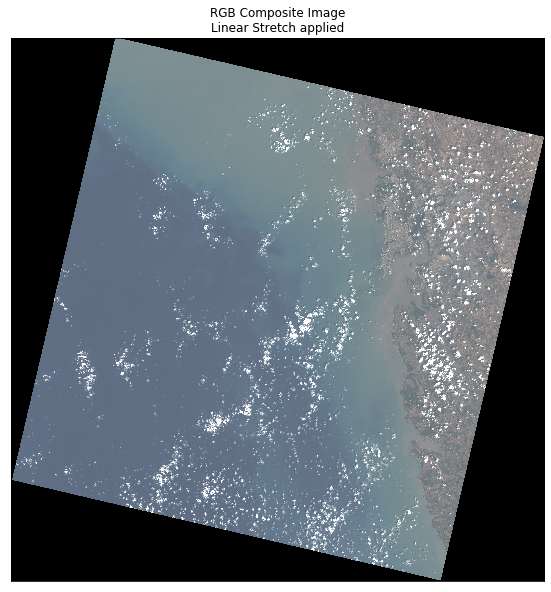
True Color Image
Using the Red, Green and Blue bands from the Landsat imagery, create a true colour (RGB) image to visualize the scene.
Output:
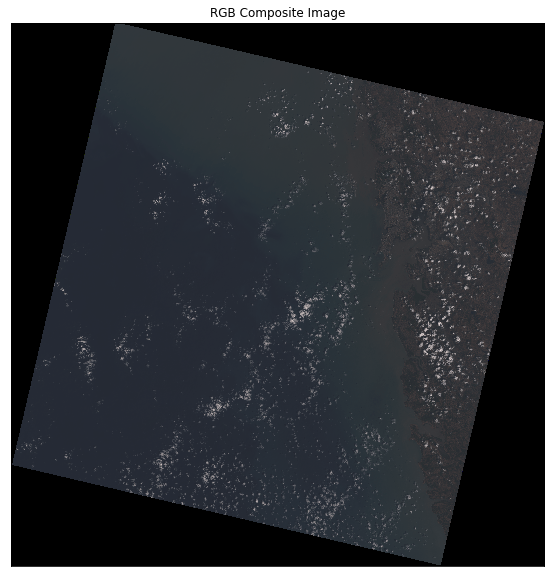
The image looks very dark because of the lack of light. Let's apply the linear stretch to brighten the image
Output:
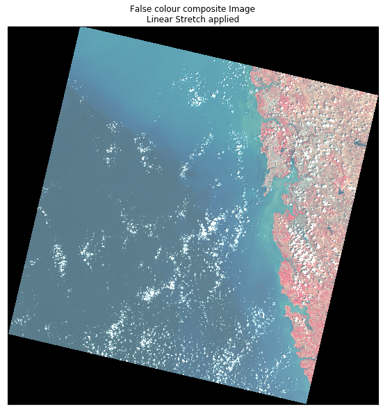
False Colour Composite Images
False colour composite images are used to visualize wavelengths that are not visible to the naked eye. Here, we visualize infrared bands along with red and green bands to see the vegetation in the scene.
Output:
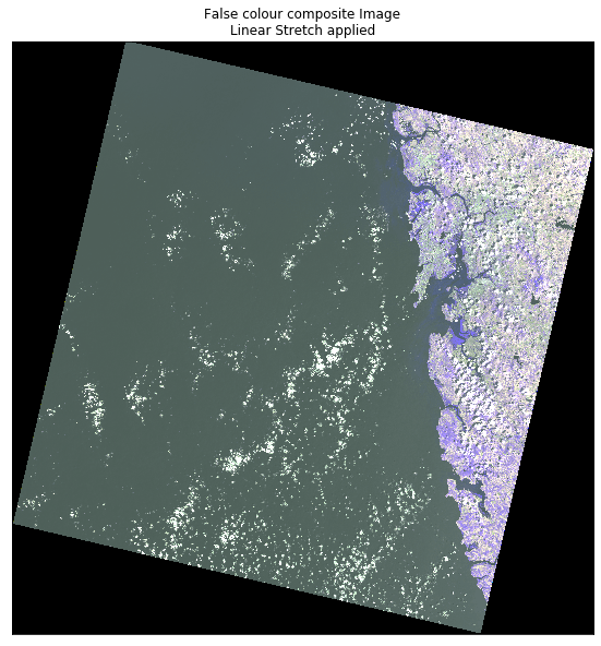
In another false colour composite image, we use NIR, SWIR and red bands to visualize the Landsat imagery in infrared.
Output:
Reference links to explore more details on Landsat Satellite imagery.
- Landsat Data Access
- Landsat 8 OLI/TIRS Level-1 Data Products
- Landsat Open Data on AWS
- Landsat Applications and Case studies
If you liked the blog, subscribe to the blog now and get notified about future blog posts. Also, comment below for any questions or suggestions. Stay tuned for the next blog of this series on Sentinel 2. Find me on LinkedIn, Twitter for any queries or discussions. Check out my previous blog on Why Geospatial Data is the way forward in data analytics here.

Do you like our stuff? Subscribe now.
Join the Pack!
Liked the content on this page? Get my articles & new insights right in your inbox. Subscribe to join many other readers.

An error has occurred somewhere and it is not possible to submit the form. Please try again later or contact us.
You may also like


.jpg)

An error has occurred somewhere and it is not possible to submit the form. Please try again later or contact us.

PGP Fingerprint
0F91 E5FA E34B 1691 C77E 8CD1 4CD2 C87C 22FE 39B9